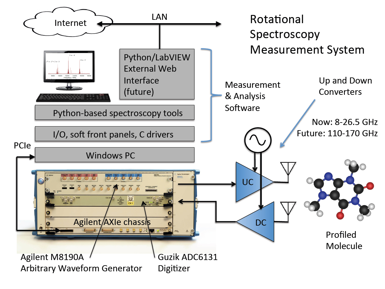
Chirped-Pulse Fourier Transform Microwave Spectroscopy

Final technical report on “Next Generation Spectrometers for Rapid Analysis of Complex Mixtures”

Dr. Steven Shipman
Division of Natural Sciences
New College of Florida
May 29, 2014

Overview

This report is the final technical report for the proposal “Next Generation Spectrometers for Rapid Analysis of Complex Mixtures”. The primary goal of this proposal was to build a spectrometer operating from 110 – 170 GHz with combined improvements in speed, sensitivity, and bandwidth of a factor of 100,000 over our previous spectrometer. This goal can be met by using a new real-time digitizer and by exploiting the fact that molecular signals are tied to the Boltzmann distribution, which peaks at mmwave frequencies for typical volatile compounds at room-temperature.

The basic operating principles of the instrument are sound. The real-time digitizer works as expected and it is possible to rapidly obtain high signal-to-noise ratio data on molecular samples at mm-wave frequencies. Full expected performance was not reached during the sample cell miniaturization work, however, and the reasons for this are discussed below. The primary limitations for this instrument design at present come both from the low available output power from the mm-wave amplifier, as well as the low power-handling capability of the mm-wave receiver.

Background Information

Molecules have internal motions that are characteristic of their structure and identity. These motions can be studied by spectroscopy in different regions of the electromagnetic spectrum. Molecular spectra can be used as a “fingerprint” to unambiguously state whether or not a particular chemical is present and in what amount. As such, small portable spectrometers are frequently used as components of chemical sensors. Chemical sensors have wide utility and are used in fields as diverse as environmental and air quality monitoring, detection of hazardous gases and chemical warfare agents, and breath analysis in medical applications. Because of this wide range of applicability, improvements to the performance and sensitivity of chemical sensors can have impacts in many different areas.

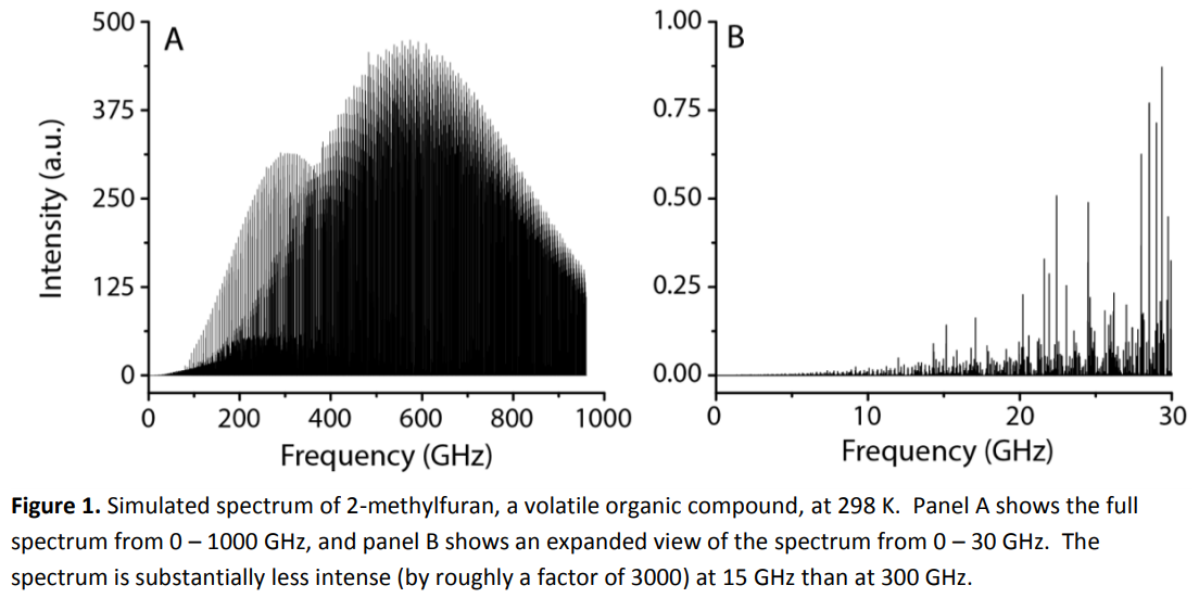
The spectrometers described here are used to study rotational motions of molecules. In principle, rotational spectroscopy can be used to detect any chemical compound with a dipole moment. (Nearly all molecules have dipole moments; the exceptions are compounds composed of just one type of atom, like O2 or N2, or molecules with a high degree of symmetry, such as benzene or C60.) Rotational spectra have traditionally been collected in the microwave / cm-wave region of the spectrum (2 – 50 GHz) at low temperatures (1 – 5 K). Achieving such low temperatures requires large, bulky instrumentation that is ill-suited for small, portable devices. Operation at room-temperature significantly relaxes these requirements, but comes at the cost of signal intensity at cm-wave frequencies, meaning that optimal sensitivity will be obtained at mm- or submm- frequencies, from 100 GHz to 1 THz (Figure 1).

The goal of this project, therefore, was to develop a fast mm-wave spectrometer that is amenable to miniaturization. The work was done in three main steps. First, a new FPGA-based digitizer that can average molecular signals in real time was used to improve data throughput to allow for the acquisition of very large numbers of averages. Second, a chirped-pulse mm-wave spectrometer was constructed using x12 amplified multiplier chains (AMCs) to generate mm-wave radiation from cm-wave sources and to detect it via heterodyne mixing with a cm-wave local oscillator. Third, schemes to reduce the size of the spectrometer sample cell were tested.

Results

Note: Subsection A, about real-time digitizer performance, is taken from the interim report on this project with only minor editorial changes, as the digitizer was thoroughly characterized when that report was submitted. Results that were found after the interim report was submitted are described below in subsections B (110-170 GHz spectrometer characterization) and C (sample cell miniaturization).

A) Real-time digitizer performance

Initial work with the real-time digitizer (Guzik ADC6131) focused on characterizing its speed and phase stability by using it as the digitizer in our existing cm-wave spectrometer. The speed of the digitizer met spec and was far beyond that of our previous instrument (Tektronix TDS6154C). The new digitizer can acquire 1 million averages of a 10 us trace, sampled at 40 GS/s (record length of 400,000 points), in just under 12 seconds. By comparison, it would take the Tektronix digitizer roughly 29 hours to collect and average the same amount of data. The new digitizer has thus given us a speed enhancement of roughly a factor of 8,750.

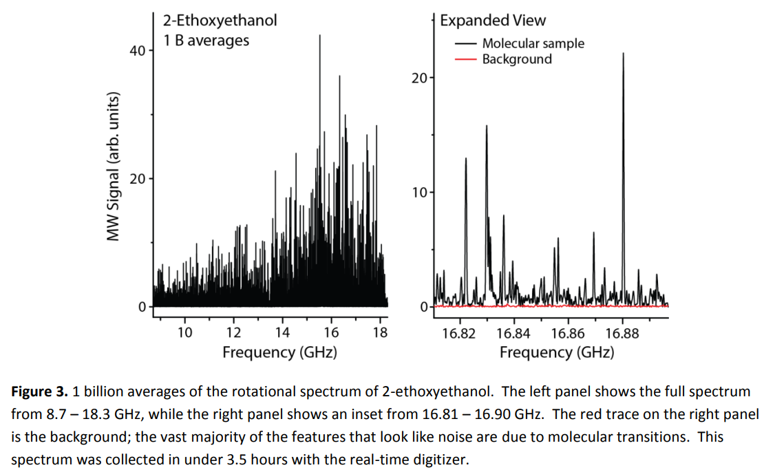
Once the speed enhancement was confirmed, we tested the phase stability of the digitizer by collecting 1 and 100 million averages of a molecular sample (nitromethane) and verifying the expected factor of 10 improvement in signal-to-noise ratios (Figure 2). We have since collected out to 1 billion averages on other samples (Figure 3). Again, these measurements, which only took 3.3 hours, would have been previously impossible, as they would have required in excess of 5 years of continuous averaging.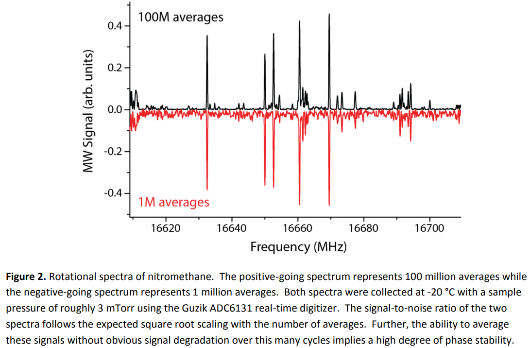

An issue that arose with these large numbers of averages was the presence of spurious coherent signals arising from the internal architecture of the real-time digitizer. Specifically, the instrument consists of 160 separate internal ADC chips, each of which acquire a signal every 4 ns, with relative offsets of 25 ps (e.g. a total 40 GS/s sampling rate when they are combined). The individual ADCs are not perfectly matched, and so they exhibit coherent internal beating patterns which manifest as spurious signals at 250 MHz increments (Figure 4A). These can be partially mitigated by acquiring a 160 point segment known to have no molecular signal at the beginning of each acquisition and then simply subtracting it from the rest of the spectrum. This reduces the magnitude of the spurs by roughly an order of
magnitude, but does not completely eliminate them (Figure 4B).

To further attenuate the spurious components, a time-domain signal processing approach can be used, making use of the fact that these signals have constant amplitude with time (unlike molecular signals, which decay exponentially). The real and imaginary parts of each spurious component can be determined from the time-domain data (at the beginning of acquisition, before a molecular signal is present) and then subtracted prior to performing the Fourier transform. This leads to another substantial reduction of the spurious components (Figure 4C).

B) 110 – 170 GHz spectrometer characterization

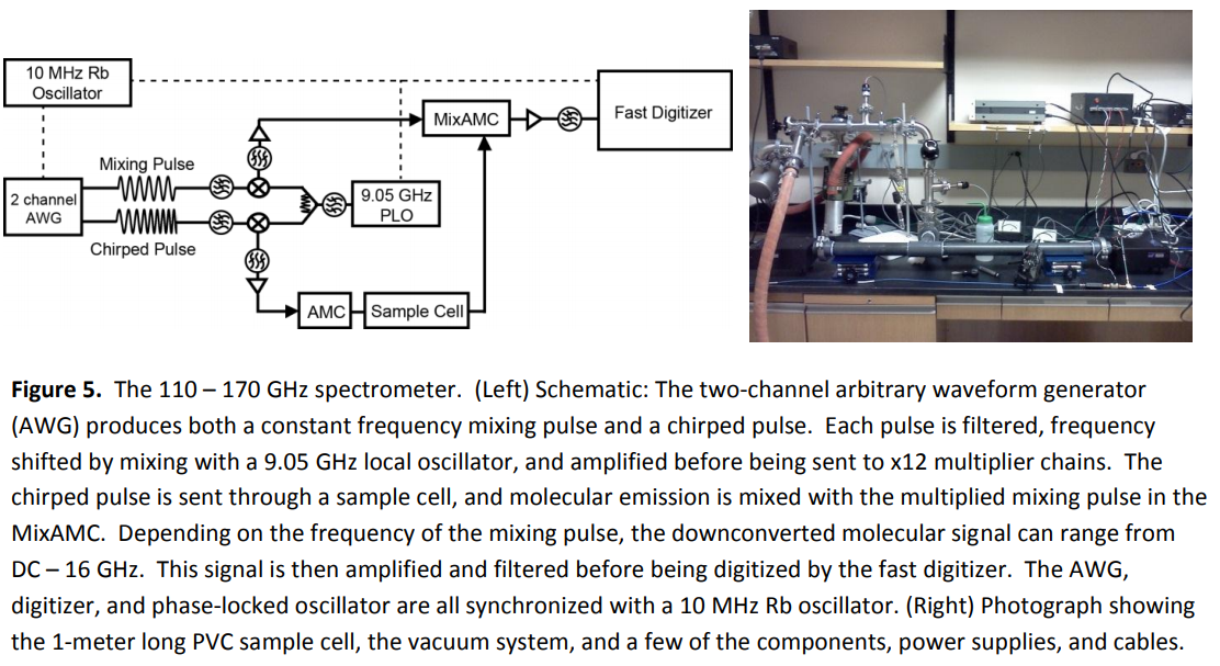
After completing digitizer testing in the cm-wave range, the 110-170 GHz spectrometer was assembled and tested. A schematic of the instrument is shown in Figure 5. A two-channel arbitrary waveform generator (Agilent M8190A) generates both a chirped pulse and a constant frequency signal to be used in the receiver. The output of each channel is filtered with a 5 GHz low-pass filter before being frequency shifted into the 9.16 – 14.16 GHz range with a double-balanced mixer and a 9.05 GHz phaselocked oscillator. The RF output from each channel is then amplified and further filtered. The chirped pulse is then sent to an x12 amplified multiplier chain (AMC), which can produce an average of roughly 7 mW of power from 110 – 170 GHz. The resulting chirped mm-wave pulses from the AMC are sent into a sample cell with Teflon lenses that both focus the light and serve as pressure windows on either end. The chirped pulses interact with molecules in the sample cell, which subsequently emit a mm-wave free induction decay (FID). The molecular FID is then mixed with the (frequency shifted, amplified, filtered) constant frequency output of the arbitrary waveform generator in an x12 mixer / amplified multiplier chain (MixAMC). This produces an IF signal that can range from DC – 16 GHz, depending on the local oscillator frequency. The IF output is then amplified and digitized by the Guzik ADC6131 digitizer.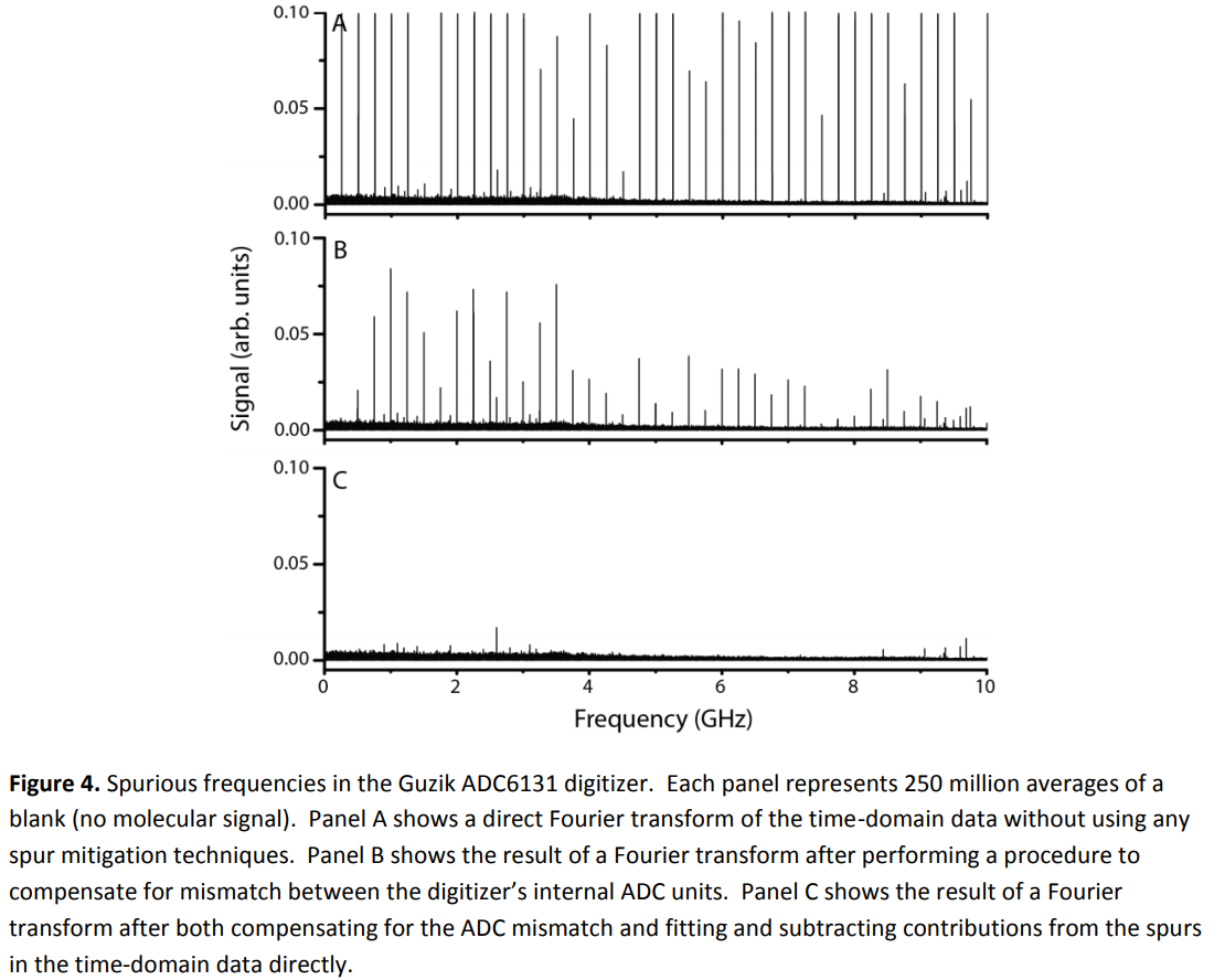

Prior to collection of molecular data, mm-wave chirped pulses were generated and characterized via spectrograms, a few of which are shown in Figure 6. Pulses can be generated and detected across most of the 110-170 GHz band, though there are some obvious variations in the amplitude of the detected pulses with frequency. The pulse quality is best between 121 and 167 GHz giving roughly 45 GHz of usable bandwidth. Frequencies that are between 110 – 120 GHz post-multiplication correspond to AWG frequencies between 0.12 and 1 GHz. Poor pulse quality in this range after the AMC appears to be due to second harmonic output from the AWG which interferes with the frequency multiplication process. The second harmonic frequencies cannot simply be filtered out because they are also in our desired passband at the stage where they are generated. The most effective way to eliminate this problem would likely be to work with a phase-locked oscillator at a lower frequency than our current 9.05 GHz, to shift the desired AWG output farther away from DC.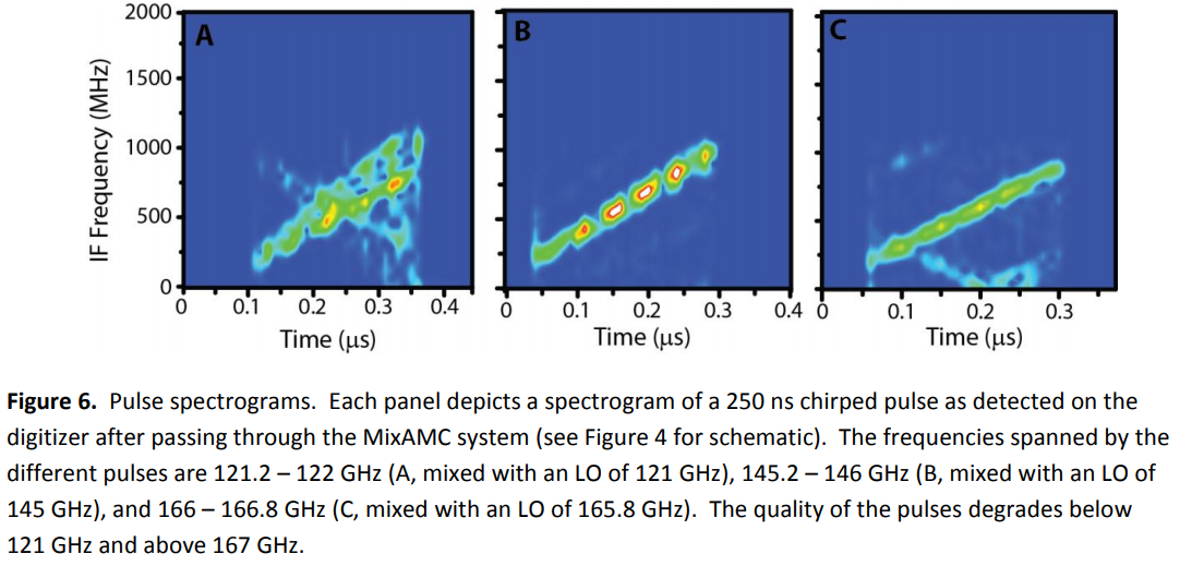

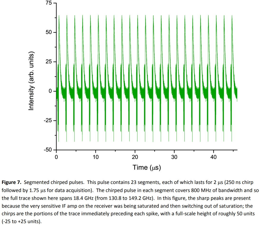
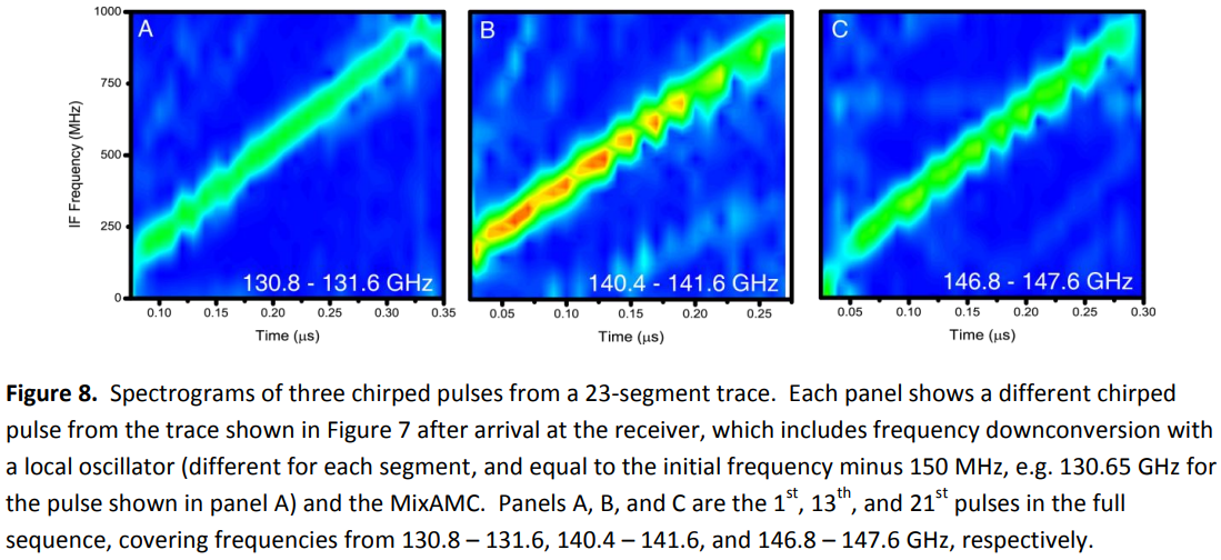
A difficulty faced with mm-wave operation is that the available output powers are far less than those obtainable at cm-wave frequencies. For example, the x12 AMC used in this work, which has an output power of roughly 7 mW, is twice as expensive as a cm-wave solid-state amplifier with an output power of 10 W. As a consequence of these relatively low powers at mm-wave frequencies, it is not possible to collect a multi-GHz spectrum using a single chirped-pulse. Instead, the best way to collect a broad spectrum is to do so over a series of short segments, each covering only a small bandwidth to make good use of the limited available power. In segmented operation, a short excitation pulse is sent through the sample and followed by a period of data collection. This is repeated for each segment. Figure 7 shows a digitizer trace containing 23 segments, each spanning 800 MHz, covering a total bandwidth of 18.4 GHz. Each repetition of the full trace is acquired in just over 46 us (2 us per segment, plus a short dead time at the beginning of the acquisition). Figure 8 shows spectrograms of the 1st, 13th, and 21st chirps at the receiver (after mixing with their respective local oscillator frequencies), showing that each pulse is relatively clean.

While performing the multi-segment tests, we uncovered a bug in the digitizer software which did not allow access to the full memory (this issue is why the trace in Figure 7 is only 46 us in duration). This has been remedied, and a new version of the firmware allows use of the full memory range. At a sampling rate of 2.5 GS/s, this would allow an individual trace to be 128 us long. If 64 segments of 2 us are used, each covering 800 MHz of bandwidth, this would allow for a total bandwidth of 51.2 GHz, which is essentially the entire useable range of the mm-wave components in this spectrometer. The 2.5 GS/s sampling rate would constrain us to an upper frequency of 1.25 GHz at the receiver via the Nyquist limit, but this is perfectly fine if each chirped pulse only covers 800 MHz of bandwidth.

Once chirped-pulse generation and detection were tested, we used methanol to find optimal conditions for spectrum collection. Peak intensities and therefore overall spectrometer sensitivity depend on several factors. The most straightforward to vary experimentally are the properties of the excitation pulse (bandwidth and duration) and the sample pressure. The pulse bandwidth and duration determine the amount of energy delivered to the sample over a given frequency region. The pulse duration needs to be kept short, as the molecular signal decays exponentially with a fast time constant. We found that a 250 ns pulse followed by data collection for 1.75 us was optimal. From there, we examined the effects of bandwidth. Higher bandwidth pulses lead to broader frequency coverage but weaker signals. To determine a baseline sensitivity to be used in later sample cell miniaturization experiments, we used a chirped-pulse that spanned 200 MHz.

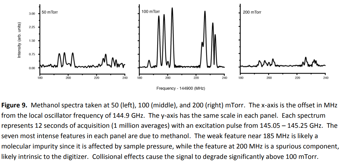
With those parameters set, we optimized the sample pressure. Figure 9 shows the methanol spectrum between 145.08 and 145.14 GHz at pressures of 50, 100, and 200 mTorr. The signals are strongly pressure-dependent; the intensity falls off rapidly at high pressures due to collisions between molecules that shorten the dephasing time. Some sensitivity at higher pressures can be regained (Figure 10) if a shorter time segment is Fourier transformed, though this comes at the cost of transition linewidth. Depending on overall goals, it may be better to opt for higher pressures and somewhat reduced sensitivity, as lower pressures reduce vacuum requirements and shorter acquisition times allow for more frequency segments to be collected in a given measurement.

C) Sample cell miniaturization

Once suitable conditions for collecting methanol signals were determined, we began work on reducing the size of the sample cell. More details are below, but in short, these tests were unsuccessful. The reason for this was unexpected – despite the fact that the x12 AMC and x12 MixAMC are designed to be used in conjunction with each other, the MixAMC has a damage threshold well below that of the typical output power of the AMC. As such, when using these components, a minimum distance between source and receiver is required to avoid damage, putting a much larger size limit on the sample cell than expected. Further, even while observing precautions to stay below the damage thresholds of the mmwave components, they were nevertheless damaged as part of the sample cell miniaturization tests before useful data could be obtained. Virginia Diodes (the manufacturer of the devices) is currently investigating the components to try to understand how they were damaged in these tests.

As mentioned earlier, the typical output power of the AMC is roughly +8.5 dBm. The damage threshold for the MixAMC, however, is +0 dBm. In the initial sample cell configuration, the AMC output was sent through a 22 dBi gain horn into a 1 meter stainless steel sample cell. The windows on both ends of the cell were plano-convex Teflon lenses of 2” diameter with a 50 cm focal length. The MixAMC collected the mm-wave frequencies through a second 22 dBi gain horn. Using the free-space path loss equation at 145 GHz and accounting for the horns but not for the Teflon lenses, the MixAMC should have seen roughly -24 dBm of power. It is difficult to estimate the performance in this frequency range of the Teflon lenses in dBi as they have only been characterized at 500 GHz, but given that the system operated successfully over extended periods when using these lenses with the 1 meter sample cell, it seems safe to assume that together they do not significantly exceed a gain of 24 dBi.

The sample cell is composed of several stainless steel segments held together with quick flange connections. The initial plan was to simply remove one of these segments and assess how much that affected methanol signal levels relative to those obtained with the initial cell length. Unfortunately, we were not able to successfully obtain any signal with a reduced-length sample cell, as the mm-wave components failed during our initial measurements. We have consulted with engineers at Virginia Diodes, who did not believe that our test should have damaged the devices. However, they did indicate that there are occasions when these components can simply fail unexpectedly. They are currently evaluating the devices to see if they can determine the source of the problem.

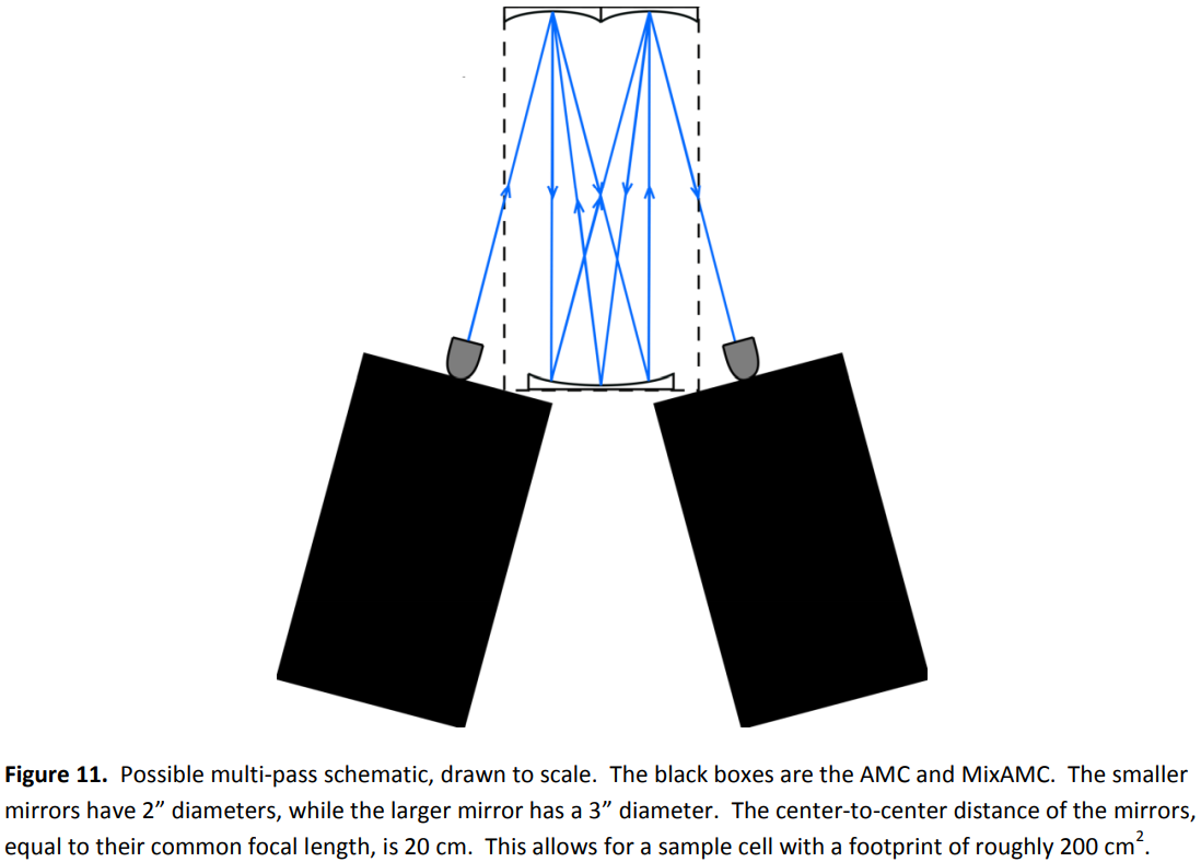
Even though the MixAMC may not have failed due to its damage threshold, it nevertheless seems clear that simply going to a short path length could be dangerous. A safer alternative would be to move to a multi-pass geometry such as the one shown below in Figure 11, based on a White cell design. This setup consists of three concave mirrors, each of the same focal length, with the mirror centers on each side separated by the common focal length. This allows for the light to make numerous passes through the sample, with the number of passes adjustable by altering the angle of the incident light. This configuration can lead to a large pathlength over several passes (and so should be safe in terms of the MixAMC damage threshold) but provides a compact footprint for the sample cell. Figure 11 is drawn to scale; the two smaller mirrors have 2” diameters, the larger mirror has a 3” diameter, and the focal length of each mirror is 20 cm. The total footprint occupied by the geometry shown in Figure 11 is then approximately 200 cm2 (20 cm length x 10 cm width), which is more than twice as small as the current setup, which is a 1 meter length tube with a diameter of 2”, giving a footprint of roughly 500 cm2 (100 cm length x 5 cm width) with an unwieldy long dimension. Real-world testing would need to be done to assess how feasible this configuration is, as it is unclear how quickly the spot size of the mmwave light will increase, which would place an upper limit on the number of passes that could be made through the cell.

Summary and Future Possibilities

Overall, this project had three primary goals. The first was to incorporate real-time digitizers into spectrometers to drastically increase data throughput. The second was to construct a mm-wave spectrometer using this technology to benefit from the natural thermal population of molecules at room temperature. The third was to then use these combined benefits to explore reductions in sample cell volume for future miniaturization efforts. The first goal was definitely met and the digitizer performance was excellent. We were able to collect spectra of 1 billion averages over the course of a few hours, when this feat would have taken in excess of 5 years with our previous system. The second goal was met, but with some caveats. Output power limitations of the amplified multiplier chain forced us to use relatively low bandwidth chirped pulses to sufficiently excite the molecules, which in turn meant that we were not able to cover the full 60 GHz bandwidth with each repetition cycle as we had initially hoped. The third goal was not met, due in part to the fragility of these devices and possibly due to the low power handling ability of the mm-wave receiver, which has a damage threshold below that of the typical output power of the amplified multiplier chain. Given that, simple reductions in pathlength are likely to put equipment at risk, but multi-pass designs that have longer effective pathlengths but reduce instrument footprint are likely the best route. Moving forwards, the two most critical areas for further development of this approach will be 1) increasing the output power of the multiplier chains at mm-wave frequencies and 2) improving the power handling of the receiver components. Without advances in these two areas, it will be very difficult to meet the goal of building a small, field-portable instrument that can efficiently cover large bandwidths. That being said, even with current capabilities, there are still interesting possibilities to explore. In particular, given the extreme flexibility of the arbitrary waveform generator used in this design, there is no reason that adjacent segments in a multi-segment trace need to have continuous frequencies. For instance, if one is interested in monitoring levels of 20 different gases, it would be straightforward to use a 20 segment trace in which each segment covers a particular frequency range where a unique spectral signature for each gas is likely to be found, with no direct connection between the frequencies covered in the various segments. Once the cause of failure on the mm-wave components has been diagnosed and they are repaired, we plan to explore this avenue further.